The Integral of Noise in State Estimation
Table of Contents
Introduction
Noise modeling is a crucial component of probabilistic state estimation. Suppose you have a non-holonomic wheeled robot with two noisy sensors. One measures yaw rate, and the other measures forward speed. To estimate position via dead-reckoning, one can integrate these signals through a motion model with the caveat that error will accumulate due to the integration of noise.
A Toy Problem
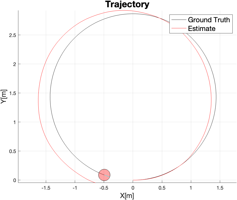
To get a better sense of this, we create a synthetic scene with a robot moving and turning at a constant rate ($v, \omega$), in a circular trajectory:
$$
\begin{align*}
v = 0.5m/s&, \omega = 20deg/s\\
\mathbf{X}(t) &= \left[\begin{matrix}x(t)\\y(t)\\\theta(t)\end{matrix}\right]\\
\mathbf{\dot{X}}(t) &= \left[\begin{matrix}v\cos(\theta(t))\\v\sin(\theta(t))\\\omega\end{matrix}\right]
\end{align*}
$$
Assume we sample our sensors at a time step of $\Delta t$. To move our robot forward, we numerically integrate the motion model:
$$
\begin{align*}
\mathbf{X}_0 &= \left[\begin{matrix}0\\0\\0\end{matrix}\right]\\
\mathbf{X}_t &= \mathbf{X}_{t-1} + \mathbf{\dot{X}}_t \Delta t\\
&= \left[\begin{matrix}x_{t-1} + v\cos(\theta_{t-1})\Delta t\\y_{t-1} + v\sin(\theta_{t-1})\Delta t\\\theta_{t-1} + w\Delta t\end{matrix}\right]
\end{align*}
$$
With this motion model, we obtain the following trajectory:
Analyzing the Signals
Plotting the robot state and error against time gives us:
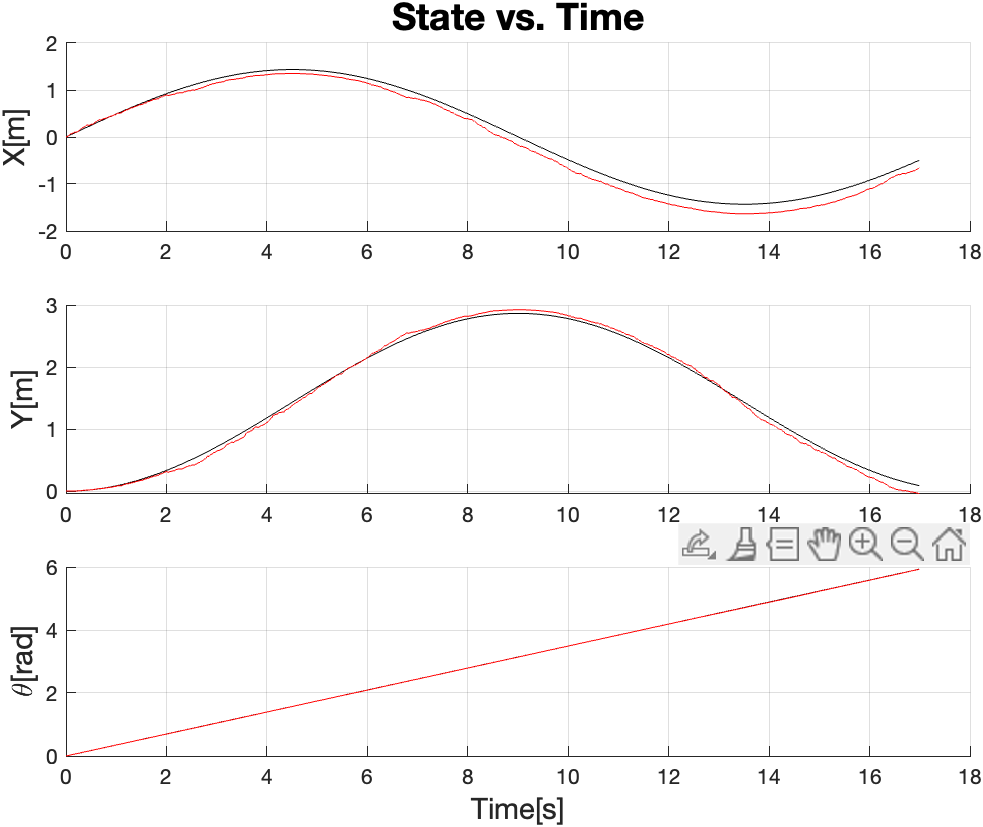
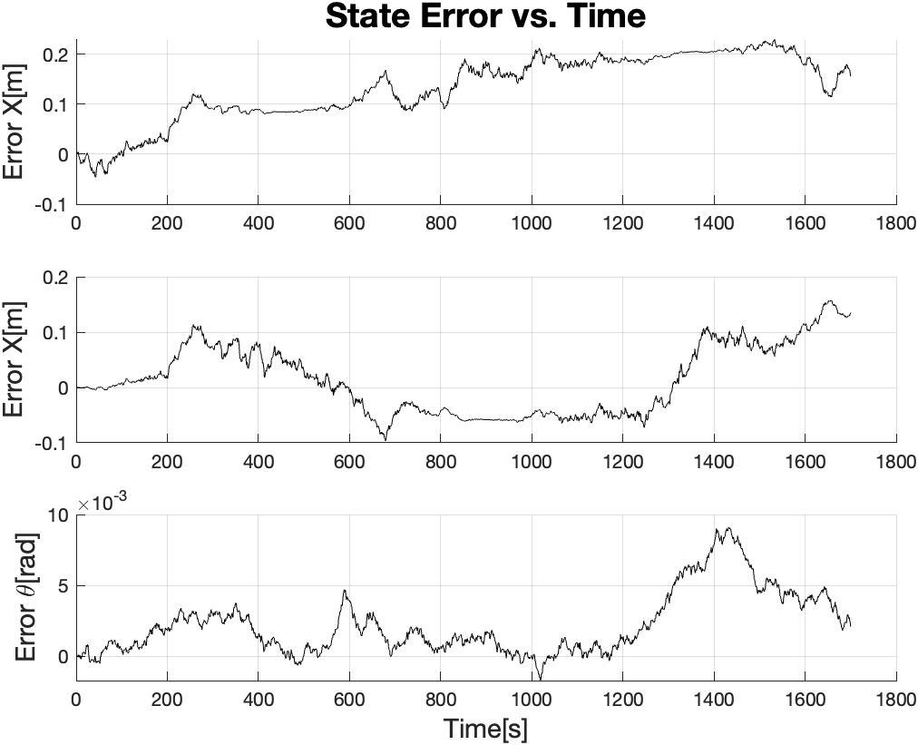
We examine the last error plot, $\epsilon_\theta(t) = \hat{\theta}(t) - \theta(t)$ where $\hat{\theta}(t)$ is our estimate at some point in time. Since we know that $\omega$ is “noisy”, we account for this in our estimate equation.
Let $w_t \sim \mathcal{N}(0, \sigma)$, i.e. some normally distributed noise value that comes tacked onto $\omega$ and some time $t$. We don’t know exactly what that value is, but we know it exists, and it’s random at every iteration.
$$
\begin{align*}
\hat{\theta}_t &= \hat{\theta}_{t-1} + (\omega + w_t)\Delta t\\
\end{align*}
$$
We expand this recursion:
$$
\begin{gather*}
\hat{\theta}_0 = 0\\
\hat{\theta}_1 = \hat{\theta}_0 + (\omega + w_1)\Delta t\\
\hat{\theta}_2 = \hat{\theta}_1 + (\omega + w_2)\Delta t = \hat{\theta}_0 + (\omega + w_1)\Delta t + (\omega + w_2)\Delta t\\
\hat{\theta}_3 = \hat{\theta}_2 + (\omega + w_3)\Delta t = \hat{\theta}_0 + (\omega + w_1)\Delta t + (\omega + w_2)\Delta t + (\omega + w_3)\Delta t\\
\cdots\\
\hat{\theta}_t = \hat{\theta}_0 + \Delta t\sum_{i=0}^t \omega + \Delta t\sum_{i=0}^t w_i
\end{gather*}
$$
Let
$$
\begin{gather*}
\theta_t = \hat{\theta}_0 + \Delta t\sum_{i=0}^t \omega\\
W_t = \Delta t\sum_{i=0}^t w_i\\
\hat{\theta}_t= \theta_t + W_t
\end{gather*}
$$
We recognize that $\theta_t$ is just the ground truth signal. $W_t$ is a new term which is the numerical integration of mean-centered Gaussian noise, $W_t$. This signal is also known as the Wiener process, the continuous analog of Brownian motion.
If you ran this simulation many times with the same noise parameters to obtained different noisy sensor signals, and plotted the error signals on top of each other, you get a group of signals such that at any given time $t$, their variance at that time is equal to $\sigma_w^2(t) = \left(\sigma^2\Delta t\right)t$. The standard deviation is thus $\sigma_w(t) = \left(\sigma\sqrt{\Delta t}\right)\sqrt{t}$.
The animation below illustrates this. Note how the red curve ($\sigma_w$ measured at that particular moment in time across all measurements) slowly converges to the green curve as the number of samples increases.
Note that the units of measure of $\sigma_w$ are $rad/\sqrt{s}$ which is equivalent to $\frac{rad}{s} / \sqrt{Hz}$. This makes intuitive sense because it’s the rate at which the square-root of uncertainty increases as you integrate the signal.
Notes
In a Kalman filter, the propagation step is a two-step process:
- Integrate your inertial sensors to dead-reckon your next state.
- Increase your state uncertainty proportional to your integrated sensor noise.
What you are effectively doing is keeping track of both what the raw numerically integrated state looks like, and also keeping track of the size of the envelope in which your state actually is.
Note, if you have a state variable that integrates another state variable that integrates sensor noise (e.g. position integrates velocity which integrates accelerometer data), your uncertainty for that state variable grows quadratically.
The AR(1) Model
The Wiener process is a signal that can grow unboundedly. Sometimes, it is useful to have a model for a noise signal that has a bounded uncertainty. For instance, GPS signals can drift by many meters even while stationary. However, often times your GPS signal will typically meander about its resting position. Such a signal can be modeled by an auto-regressive model.
A common one is the AR(1) process:
$$ \begin{gather*} y_t = \rho y_{t-1} + w_t \end{gather*} $$
This equation is very similar to the Wiener process, except during the integration, the prior value of the random walk is scaled by $\rho$. When we expand the recursion out, we get the following:
$$
\begin{gather*}
y_0 = 0\\
y_1 = \rho y_0 + w_1 = \rho w_0 + w_1\\
y_2 = \rho y_1 + w_2 = \rho^2 w_0 + \rho w_1 + w_2\\
y_3 = \rho y_2 + w_3 = \rho^3 w_0 + \rho^2 w_1 + \rho w_2 + w_3\\
y_t = \left(\sum_{i=0}^t\rho^{t-i} w_i\right) + w_t
\end{gather*}
$$
We examine the effect of $\rho$ on this signal:
- When $\rho = 0$, the random walk portion is immediately zero’d out: $y_t = w_t$. This is equivalent to no time correlation, i.e. white noise.
- When $\rho = 1$, this is a standard Wiener process if you were to scale $w_k$ by $\Delta t$.
- When $\rho > 1$, the previous sample gets amplified exponentially at each iteration by a factor of $\rho$. This signal explodes very quickly over time.
We’re thus only interested in the case of $0 < \rho < 1$ where each prior random walk signal is attenuated. In this case, $\rho$ can be thought of as some damping factor.
Assuming $0 < \rho < 1$, we recognize that $\sum_{i=0}^t\rho^{t-i}w_i$ is a
geometric progression. The variance of this signal is thus:
$$
\begin{align*}
Var\left[y_t\right] &= \sigma^2\lim_{t\rightarrow \infty}\sum_{i=0}^t\left(\rho^{t-i}\right)^2\\
&= \sigma^2\left(1 + \rho^2 + \rho^4 + \dots\right)\\
&= \sigma^2\frac{1}{1-\rho^2}
\end{align*}
$$
This is interesting because we can see that as the signal progresses forever, the variance is bounded, unlike the Wiener process where the random walk can meander to infinity over time. The AR(1) process ensures that the random walk generally stays within some soft radius of its mean value, making it perfect for modeling things like GPS drift.
To ensure this $0 < \rho < 1$ constraint, we parameterize $\rho$ as the following: $$ \rho = e^{-\Delta t/\tau} $$
where $\tau$ is some “time constant”. The variance follows the continuous time form: $$ Var\left[y(t)\right] = \sigma^2\frac{1}{1-\rho^2}\left(1 - e^{-2t/\tau}\right) $$
The animation below illustrates this.